Directional Loads
For most directional loads and supports, their directions can be defined in any coordinate system:
The coordinate system must be defined before applying the load, and the direction of loads and supports can only be defined in a Cartesian coordinate system.
In the Details view, change “Define By” to “Components” and select the appropriate Cartesian coordinate system from the dropdown menu.
Specify the x, y, and z components in the selected coordinate system.
Not all loads and supports support the use of coordinate systems.
Acceleration (Gravity)
Acceleration is applied to the entire model in units of length per time squared.
Users often find the direction of acceleration confusing. If acceleration is applied suddenly, inertia resists changes, so inertia force acts opposite to the direction of acceleration.
Acceleration can be applied through components or vectors.
Standard Earth gravity can be applied as a load, with a value of 9.80665 m/s².
The direction of standard Earth gravity can align with any axis of the global coordinate system, but gravity must be defined opposite to its actual direction to simulate the gravitational force.
Rotational velocity:
Rotational velocity is another form of inertial load:
The entire model rotates around a specified axis at a given speed.
It can be defined by a vector or by applying the axis and rotational speed based on the geometry.
Components can define rotational velocity, specifying initial and constituent parts in the global coordinate system.
Pay close attention to the rotation axis.
Default rotational velocity is given in radians per second, but this can be changed to revolutions per minute (RPM) under “Tools > Control Panel > Miscellaneous > AngularVelocity.”
Pressure Load
Pressure can only be applied to surfaces and is typically aligned with the surface normal.
Positive values indicate pressure applied to the surface (e.g., compression), while negative values indicate suction or removal from the surface.
The unit of pressure is the force per unit area.
Force Load
Force can be applied to the outermost surfaces, edges, or structure.
The force will be distributed throughout the structure, meaning that if applied to two identical surfaces, each will experience half the force. The unit of force is mass times length divided by time squared.
Forces can be applied by defining vectors, magnitudes, and components.
Bearing Load
Bolt loads are only applicable to cylindrical surfaces. The radial components distribute pressure loads based on the projected area, while the axial load is evenly distributed along the circumference.
A cylindrical surface can only receive one bolt load. If the surface is divided, both sections must be selected when applying the bolt load.
The unit of load is the same as force.
Bolt loads can be defined by vectors, magnitudes, or components.
Torque Load
For solids, torque can be applied to any surface.
If multiple surfaces are selected, the torque is distributed among them.
Torque can be defined using vectors, magnitudes, or components. When using vectors, the right-hand rule applies.
Torque can also be applied at vertices or edges of a solid surface, similar to surface-based torque defined by vectors or components.
The unit of torque is force multiplied by length.
Off-Center Load
Allows the application of a biased force on a face or edge.
The user sets the initial position of the force (using a vertex, circle, or x, y, z coordinates).
Force can be defined using vectors, magnitude, or components.
This results in an equivalent force on the surface, along with a moment caused by the biased force.
The force is distributed across the surface but includes the moment due to the offset force.
The unit of force is mass * length / time².
Bolt Load
Preload is applied to simulate bolt connections on cylindrical surfaces.
Preload (force) or displacement (length) is set as the initial condition.
Sequential loading allows additional options; preload is applied in the initial solution, and other loads are applied in subsequent steps.
Bolt connections can be automatically locked in the second step.
Only applicable in 3D simulations, with a local coordinate system required for entities.
Element refinement is recommended for bolts (with more than one element along the bolt length).
Constrains all degrees of freedom at vertices, edges, or faces.
For solids, restricts x, y, and z translations.
For shells and beams, restricts translations and rotations.
Prescribed Displacement:
Allows specifying known displacements at vertices, edges, or faces.
Forcibly applies displacement in x, y, and z directions.
“0” input indicates constraint in that direction.
Frictionless Constraint:
Applies normal constraints on surfaces.
For solids, it can be simulated using symmetric boundary conditions.
Cylindrical Surface Constraint:
Applied to cylindrical surfaces, allowing axial, radial, or tangential constraints.
Only applicable for small deformation (linear) analysis.
Compression-Only Constraint:
Limits movement to compression along the surface’s normal direction.
Often used in simulations with non-linear solvers to determine compression behavior.
Simple Constraint:
Applied to edges or vertices of beams or shells.
Restricts translation, but rotation remains free.
Fixed Rotation:
Applies to surfaces, edges, or vertices of shells or solids.
Restricts rotation, but allows translation.
Summary:
Constraints and contact pairs define boundary conditions. Contact pairs simulate “flexible” boundary conditions, while fixed constraints provide “rigid” conditions without modeling rigid parts.
Type of Support
Equivalent Contact Condition at Surfaces of Part
Fixed Support
Bonded contact with a rigid, immovable part
Frictionless Support
No Separation contact with a rigid, immovable part
Compression Only Support
Frictionless contact with a rigid, immovable part
If you’re interested in the connection between parts A and B, consider whether both parts need to be analyzed (via contact) or if applying a fixed constraint to part B relative to A is sufficient.
In other words, is part B “rigid” compared to A? If so, you can simulate only a fixed constraint on part A. If not, you will need to simulate friction between the two.
Thermal Load: In a model, temperature causes thermal expansion.
Thermal strain is calculated as follows:
Where α is the coefficient of thermal expansion (CTE), T_ref is the reference temperature when thermal strain is zero, T is the applied temperature, and ε_th is thermal strain.
Thermal strain itself doesn’t cause stress, but stress can arise when constraints, temperature gradients, or mismatched thermal expansion coefficients are present.
CTE is defined under the “Engineering” dropdown menu, with units of strain per unit temperature.
Thermal loads can be applied to the model:
Any temperature load can be applied.
DS typically performs thermal analysis first, and then inputs the resulting temperature field as a load in structural analysis.
Assembly - Solid Contact
When inputting an assembly of solids, contact is automatically generated between two solids.
Face-to-face contact allows mismatched element divisions on the boundaries of the two solids.
Users can control the tolerance by adjusting the slider for detecting automatic contact distance in the “Contact” menu.
In DS, each contact pair must define the target and contact surfaces.
One surface of the contact area forms the “contact” surface, and the other forms the “target” surface.
Penetration of the target surface (within a given tolerance) limits integration points on the contact surface. The opposite case is incorrect.
Asymmetric Contact: One surface is the target, the other is the contact surface.
Symmetric Contact: Both surfaces are either contact or target surfaces, allowing penetration from either side.
By default, DS defines symmetric contact. Users can change it to asymmetric contact based on the description above for ANSYS Professional licenses and structural modules.
Four types of contact are available:
Column 1
Column 2
Column 3
Column 4
Contact Type
Iterations
NormalBehavior (Separation)
Tangential Behavior (Sliding)
Bonded
1
Closed
Closed
No Separation
1
Closed
Open
Frictionless
Multiple
Open
Open
Rough
Multiple
Open
Closed
Bonded and Non-separating Contact: These are the most basic linear behaviors and require only one iteration.
Frictionless and Rough Contact: These are nonlinear behaviors that require multiple iterations, but still rely on small deformation theory assumptions.
Options can be set under the corresponding menu: “Actual Geometry (and Specified Offset)” or “Adjusted to Touch,” allowing users to adjust the gap in the ANSYS model to the ‘just touching’ position.
For advanced users, additional contact options can be modified:
The equations can be changed from “Pure Penalty” to “Augmented Lagrange,” “MPC,” or “Normal Lagrange.”
“MPC” is only applicable for bonded contact.
“Augmented Lagrange” applies to standard ANSYS models.
In bonded contact, the pure penalty method can be visualized as applying a very high stiffness coefficient between the contact surfaces to prevent relative sliding, assuming negligible relative movement.
The MPC equation defines constraint equations for the relative motion between contact surfaces, preventing mutual sliding, often seen as a better alternative to the penalty method.
Pinball Region: This can be defined and displayed to indicate locations of close-range open contact. Beyond this region is considered long-range open contact.
Initially, the pinball region was a highly effective contact detector but is also used for other purposes, such as bonded contact.
For bonded or non-separating contact, if the gap or penetration is smaller than the pinball region, it is automatically removed.
Additional advanced options will be discussed in later sections.
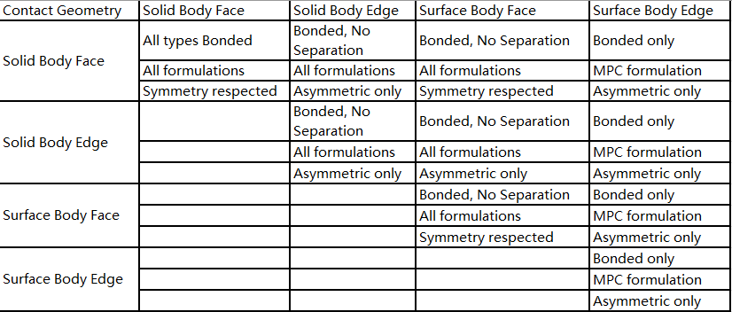
ANSYS Professional 1 licenses and above support mixed assemblies of shells and solids, allowing for complex assemblies that leverage the advantages of shells, providing more contact options and post-processing capabilities.
Edge Contact: This is a subset of generated contact, including shell faces or solid edges, only defining bonded or non-separating contact types.
For edge contact involving shell edges, only MPC form of bonded behavior can be defined.
For MPC-based bonded contact, users can set the searcher to target normals or the pinball region (which requires multi-point constraints).
If gaps exist (common in shell assemblies), the pinball region can act as a detector for contact across gaps.
A summary table of contact types and their available options in DS follows.
This table is also available in DS’s online help. It helps users decide which options are available for selection.
Weld Points:
Weld points provide a way to connect shell assemblies at discontinuous locations.
ANSYS DesignSpace licenses do not support shell contact, making weld points the only way to define a shell assembly.
Weld points are defined in CAD software and are only recognized in DS if defined in DM and UG.
Weld points can also be generated in DS, but only at discontinuous vertices.
Contact Results:
Contact results can be requested for selected entities or surfaces with contact elements.
Contact elements in ANSYS use the concepts of contact and target surfaces, with only contact elements displaying results. MPC-based contacts and edge-based contacts do not display results. Lines do not display contact results.
Asymmetric and automatic asymmetric contact will show results on the contact surface, with zero results on the target surface.
Symmetric contact will show results on both the contact and target surfaces, such as contact pressure (the average force on both surfaces).
Types of Contact Results:
Contact Pressure: displays normal contact pressure distribution.