In the physical world, differential equations are ubiquitous. They describe how fluids move, how heat is transferred, and how materials deform. Unfortunately, most differential equations are difficult to solve with elegant analytical solutions, so numerical methods are often relied upon for computation. Traditional numerical methods (such as the finite element method, finite difference method, finite volume method, etc.) have matured in solving partial differential equations (PDEs), but their computational complexity and resource consumption are often enormous when dealing with high-dimensional problems or complex geometries. Meanwhile, deep learning has shone brightly in fields like image recognition and natural language processing, leading to the question: Could neural networks be used to approximate the solutions of differential equations?
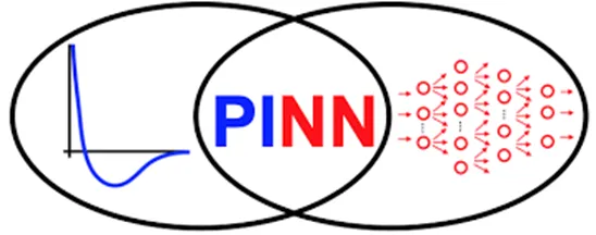
However, traditional neural networks face serious issues when handling scientific computing problems: they ignore physical laws and rely solely on data training, failing to ensure that predictions conform to basic physical principles. In this context, the concept of Physics-Informed Neural Networks (PINNs) was introduced. PINNs combine the function approximation capabilities of traditional neural networks with constraints from physical laws, directly incorporating known physical principles into the neural network training process to maintain adherence to real physical rules during training. The core idea is: during neural network training, not only is error calculated using observational data, but physical constraints are also built by introducing the governing equations, boundary conditions, and initial conditions, ensuring that the network’s output automatically satisfies these constraints. This idea was systematically proposed by scholars such as Raissi between 2017 and 2019 and quickly became a research hotspot in scientific computing and engineering simulation.
It can be simply understood like this: A traditional neural network is like a student who only memorizes by rote; as long as enough data is provided, it can remember it. But once it encounters a problem it hasn’t studied, it’s prone to errors. A PINN, on the other hand, is more like a student who not only memorizes the question bank but also masters the principles—it must pass both the “memory exam” and the “principle exam” during training. The former requires fitting observational data, while the latter requires adhering to physical laws.
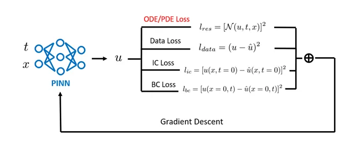
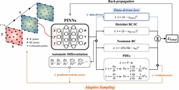
PINNs treat deep neural networks as approximate representation functions for unknown solutions. Their inputs are typically spatiotemporal coordinates (x, y, z, t), and outputs correspond to the physical quantities to be solved (such as velocity fields, temperature fields, pressure fields, etc.). During training, the loss function of a PINN usually consists of two parts: the data loss term and the physics loss term.
- The data loss term measures the error between the neural network’s predictions and observational data, ensuring the model’s fitting accuracy at known sample points.
- The physics loss term imposes constraints by substituting the network output into the governing partial differential equations (PDEs) of the system, combined with boundary and initial conditions. In practice, automatic differentiation (AD) is used to obtain the required partial derivatives, constructing equation residuals and quantifying their magnitude to ensure the neural network’s approximate solution satisfies the underlying physical laws.
By simultaneously minimizing these two loss terms, PINNs can maintain data consistency while adhering to the physical constraints implied by the governing equations, resulting in more reasonable and generalizable solutions. Thanks to this, PINNs excel in solving problems that traditional numerical methods struggle with. PINNs have been applied in various fields such as fluid mechanics, heat transfer, solid mechanics, quantum mechanics, and materials science, offering high-precision solutions for forward problems and unique advantages in inverse problems and parameter identification.
Next, let’s demonstrate how to implement the PINN algorithm through a simple heat transfer case. First, define a simple neural network structure and dataset class.
import torchtorch.manual_seed(42)

class Net(torch.nn.Module):

    def __init__(self, indim=1, outdim=1):        super().__init__()        self.actf = torch.tanh        self.lin1 = torch.nn.Linear(indim, 100)        self.lin2 = torch.nn.Linear(100, outdim)

    def forward(self, x):        x = self.lin1(x)        x = self.lin2(self.actf(x))        return x.squeeze()
from torch.utils.data import Dataset, DataLoader

class MyDataset(Dataset):

    def __init__(self, in_tensor, out_tensor):        self.inp = in_tensor        self.out = out_tensor

    def __len__(self):        return len(self.inp)

    def __getitem__(self, idx):        return self.inp[idx], self.out[idx]
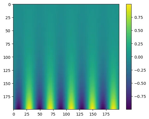
Construct the exact solution of the equation to be solved and visualize it.
import numpy as npimport matplotlib.pyplot as plt

def u(x, t):    return np.exp(-2*np.pi*np.pi*t)*np.sin(np.pi*x)

pts = 200ts = np.linspace(0.2, 0, pts)xs = np.linspace(-5, 5, pts)

X, T = np.meshgrid(xs, ts)U = u(X, T)

plt.imshow(U)plt.colorbar()
Prepare the dataset required for PINN training and define the physics loss function.
DEVICE = torch.device('cuda' if torch.cuda.is_available() else 'cpu')

train_in = torch.tensor([[x, t] for x, t in zip(X.flatten(), T.flatten())], dtype=torch.float32, requires_grad=True)train_out = torch.tensor(u(X.flatten(), T.flatten()), dtype=torch.float32)

train_in.to(DEVICE)train_out.to(DEVICE)

train_dataset = MyDataset(train_in, train_out)train_dataloader = DataLoader(train_dataset, batch_size=256, shuffle=True)

def phys_loss(inp, out):    dudt = torch.autograd.grad(out, inp, grad_outputs=torch.ones_like(out), create_graph=True, allow_unused=True)[0][:,[1]]    dudx = torch.autograd.grad(out, inp, grad_outputs=torch.ones_like(out), create_graph=True, allow_unused=True)[0][:,[0]]    d2udx2 = torch.autograd.grad(dudx, inp, grad_outputs=torch.ones_like(dudx), create_graph=True, allow_unused=True)[0][:,[0]]    return torch.nn.MSELoss()(d2udx2, 0.5*dudt)

bdry_pts = 200xs_bdry = np.linspace(-5, 5, bdry_pts)ts_bdry = np.asarray([0 for x in xs_bdry])us_bdry = u(xs_bdry, ts_bdry)

train_in_bd = torch.tensor([[x, t] for x, t in zip(xs_bdry, ts_bdry)], dtype=torch.float32, requires_grad=True)train_out_bd = torch.tensor(us_bdry, dtype=torch.float32)

train_in_bd.to(DEVICE)train_out_bd.to(DEVICE)
Build a traditional neural network model and train it. Note that the loss function at this point does not include the physics loss term.
from torch.optim import Adam, LBFGSfrom torch.optim.lr_scheduler import LambdaLRfrom torch.autograd import Variableimport torch

model = Net(indim=2, outdim=1).to(DEVICE)epochs = 1000optimizer = Adam(model.parameters(), lr=0.1)scheduler = LambdaLR(    optimizer=optimizer,    lr_lambda=lambda epoch: 0.999**epoch,    last_epoch=-1)

loss_fcn = torch.nn.MSELoss()

for epoch in range(epochs):    for batch_in, batch_out in train_dataloader:        batch_in = Variable(batch_in.to(DEVICE), requires_grad=True)        batch_out = batch_out.to(DEVICE)

        model.train()

        def closure():            optimizer.zero_grad()            loss = loss_fcn(model(batch_in), batch_out)            loss.backward()            return loss

        optimizer.step(closure)

    model.eval()    train_in_dev = train_in.to(DEVICE)    train_out_dev = train_out.to(DEVICE)    train_in_bd_dev = train_in_bd.to(DEVICE)    train_out_bd_dev = train_out_bd.to(DEVICE)

    base = loss_fcn(model(train_in_dev), train_out_dev)    phys = phys_loss(train_in_dev, model(train_in_dev))    bdry = loss_fcn(model(train_in_bd_dev), train_out_bd_dev)

    epoch_loss = base + phys + bdry    print(f"Epoch: {epoch+1} | Loss: {base.item():.4f} | {phys.item():.4f} | {bdry.item():.4f}")
Use the trained neural network model to predict the solution and visualize the prediction results.
def u_model(xs, ts):    pts = torch.stack([xs, ts], dim=1).to(DEVICE)    return model(pts)

pts = 200ts = torch.linspace(0.2, 0, pts, device=DEVICE)xs = torch.linspace(-5, 5, pts, device=DEVICE)X, T = torch.meshgrid(xs, ts, indexing="ij")X = X.TT = T.T

img = []for x, t in zip(X, T):    img.append(u_model(x, t).detach().cpu().numpy().tolist())

plt.imshow(img)plt.colorbar()
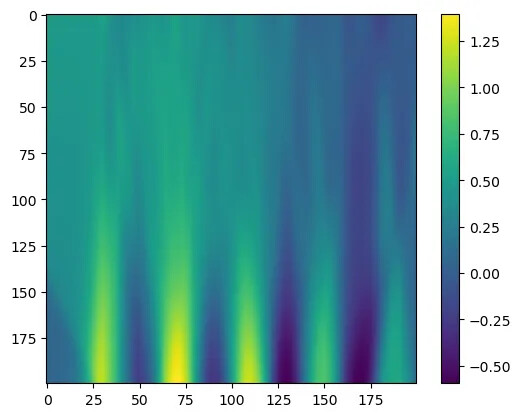
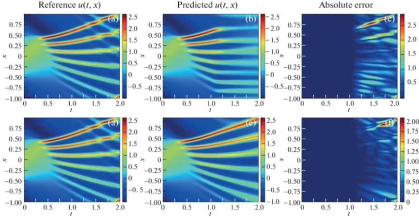
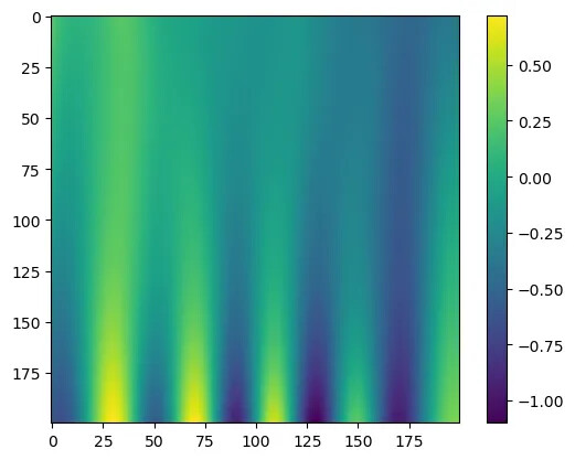
As can be seen from the above figure, the traditional neural network model, unable to understand the physical process and merely fitting the data, produces results that deviate significantly from the exact solution, and some positions do not conform to the physical equation we defined. Next, build the PINN model and train it again, this time incorporating the physics loss term into the loss function. After training, use the PINN model for prediction and visualize it.
model_pinn = Net(indim=2, outdim=1).to(DEVICE)epochs = 1000optimizer_pinn = Adam(model_pinn.parameters(), lr=0.1)scheduler_pinn = LambdaLR(    optimizer=optimizer_pinn,    lr_lambda=lambda epoch: 0.999 ** epoch,    last_epoch=-1)

loss_fcn = torch.nn.MSELoss()

for epoch in range(epochs):    for batch_in, batch_out in train_dataloader:        batch_in = batch_in.to(DEVICE).requires_grad_(True)        batch_out = batch_out.to(DEVICE)

        model_pinn.train()

        def closure():            optimizer_pinn.zero_grad()            loss = loss_fcn(model_pinn(batch_in), batch_out)            loss += phys_loss(batch_in, model_pinn(batch_in))            loss += loss_fcn(model_pinn(train_in_bd.to(DEVICE)), train_out_bd.to(DEVICE))

            loss.backward()            return loss

        optimizer_pinn.step(closure)

    model_pinn.eval()    train_in_dev = train_in.to(DEVICE)    train_out_dev = train_out.to(DEVICE)    train_in_bd_dev = train_in_bd.to(DEVICE)    train_out_bd_dev = train_out_bd.to(DEVICE)

    base = loss_fcn(model_pinn(train_in_dev), train_out_dev)    phys = phys_loss(train_in_dev, model_pinn(train_in_dev))    bdry = loss_fcn(model_pinn(train_in_bd_dev), train_out_bd_dev)

    epoch_loss = base + phys + bdry    print(        f"Epoch: {epoch+1} | Loss: {epoch_loss.item():.4f} = "        f"{base.item():.4f} + {phys.item():.4f} + {bdry.item():.4f}"    )
def u_model_pinn(xs, ts):    pts = torch.stack([xs, ts], dim=1).to(DEVICE)    return model_pinn(pts)

pts = 200ts = torch.linspace(0.2, 0, pts, device=DEVICE)xs = torch.linspace(-5, 5, pts, device=DEVICE)X, T = torch.meshgrid(xs, ts, indexing="ij")X = X.TT = T.T

img = []for x, t in zip(X, T):    img.append(u_model_pinn(x, t).detach().cpu().numpy().tolist())

plt.imshow(img)plt.colorbar()
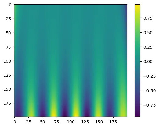
To achieve better accuracy, adopt a two-stage optimization strategy: first use Adam for coarse tuning, then LBFGS for fine tuning, balancing the model between data fitting, PDE constraints, and boundary conditions, and visualize the results.
from torch.optim import Adam, LBFGS

model_pinn_v2 = Net(indim=2, outdim=1).to(DEVICE)epochs_adam = 100epochs_lbfgs = 30optimizer_pinn_adam = Adam(model_pinn_v2.parameters(), lr=0.1)optimizer_pinn_lbfgs = LBFGS(model_pinn_v2.parameters(), lr=0.01)

loss_fcn = torch.nn.MSELoss()

train_in = train_in.to(DEVICE)train_out = train_out.to(DEVICE)train_in_bd = train_in_bd.to(DEVICE)train_out_bd = train_out_bd.to(DEVICE)

for epoch in range(0, epochs_adam + epochs_lbfgs):    current_optimizer = optimizer_pinn_adam if epoch <= epochs_adam else optimizer_pinn_lbfgs    for batch_in, batch_out in train_dataloader:

        batch_in = batch_in.to(DEVICE).requires_grad_(True)        batch_out = batch_out.to(DEVICE)

        model_pinn_v2.train()

        def closure():            current_optimizer.zero_grad()            loss = loss_fcn(model_pinn_v2(batch_in), batch_out)            loss += phys_loss(batch_in, model_pinn_v2(batch_in))            loss += loss_fcn(model_pinn_v2(train_in_bd), train_out_bd)            loss.backward()            return loss

        current_optimizer.step(closure)

    model_pinn_v2.eval()

    base = loss_fcn(model_pinn_v2(train_in), train_out)    phys = phys_loss(train_in, model_pinn_v2(train_in))    bdry = loss_fcn(model_pinn_v2(train_in_bd), train_out_bd)    epoch_loss = base + phys + bdry    print(f'Epoch: {epoch+1} | Loss: {round(float(epoch_loss), 4)} = {round(float(base), 4)} + {round(float(phys), 4)} + {round(float(bdry), 4)}')
def u_model_pinn_v2(xs, ts):    pts = torch.stack([xs, ts], dim=1).to(DEVICE)    return model_pinn_v2(pts)

pts = 200ts = torch.linspace(0.2, 0, pts, device=DEVICE)xs = torch.linspace(-5, 5, pts, device=DEVICE)X, T = torch.meshgrid(xs, ts, indexing="ij")X = X.TT = T.T

img = []for x, t in zip(X, T):    img.append(u_model_pinn_v2(x, t).detach().cpu().numpy().tolist())

plt.imshow(img)plt.colorbar()
The above is just a brief introduction to PINNs. Nowadays, AI is increasingly integrated into people’s daily lives, and the field of numerical simulation is no exception. Major simulation software companies are ramping up investments and layouts in AI projects, and traditional numerical analysis is gradually evolving toward AI-driven approaches—this trend is already quite evident. In the coming years, AI is likely to have a tremendous impact on traditional numerical simulation paradigms. However, this does not mean that traditional numerical methods will be replaced; each has its unique advantages.
It is foreseeable that the integration of AI with traditional methods will become the development direction in the field of numerical simulation.