1. Origin of Turbulence Models
1.1 From the NS Equations to the Reynolds-Averaged NS Equations
The nature of turbulence is random, chaotic, and multi-scale. In turbulent flow, the instantaneous value of any physical quantity looks like a violently fluctuating curve.
Therefore, directly solving the original NS equations, namely direct numerical simulation (DNS), requires a mesh fine enough to capture the smallest turbulent eddies. As a result, the requirements for both mesh size and time step are extremely high.
Original NS momentum equation (in index notation):
In a high-Reynolds-number region of 0.1 m × 0.1 m, the required mesh count can reach 1 billion to 100 billion cells, and the time step must be less than 100 microseconds. This is far beyond the capability of ordinary engineering calculations.

To solve this computational problem, Reynolds discovered that the curve of an instantaneous physical quantity in turbulence can actually be decomposed into two parts: a mean value and a fluctuating value:
Because the upward and downward fluctuations cancel each other out, when we average the fluctuating value, the result is always zero. This simple property is exactly the mathematical foundation of the Reynolds averaging method.
The original NS equations describe instantaneous flow. Substituting velocity and pressure as “mean value + fluctuating value” and then averaging the entire equation gives the Reynolds-averaged NS equations, namely RANS:
Compared with the original NS equations, we can see that RANS has one additional term compared with the original NS equations: the Reynolds stress term:
In other words, the RANS equations are actually more complex. So what is the purpose of taking such a long detour to transform the equations?
We transform the equations not to make their form simpler or nicer-looking, but to make them easier to solve. Although the NS equations are formally simpler, all their physical quantities are transient quantities that change at every moment, which imposes very high requirements on solution accuracy.
The unknowns in the RANS equations, however, are mean values. Mean values vary smoothly in time and space, and there is no need to capture tiny fluctuations. Their requirements for computational accuracy are much lower, so we can use coarser meshes and larger time steps to compute the RANS equations.
At the same time, what most engineering problems care about is precisely the mean flow field, such as the average velocity in a pipe or the average lift of an airfoil. Therefore, while satisfying engineering accuracy, RANS greatly reduces computational cost.
1.2 Closure Problem of the RANS Equations
We decide to use RANS. But after writing out the RANS equations, we find that the number of equations is smaller than the number of unknowns.
Original NS equations: 4 equations (mass + momentum in three directions), 4 unknowns (u, v, w, p). The equations are closed and theoretically solvable.
Continuity equation:
Momentum equation (using the x direction as an example):
(The momentum equations in the y and z directions have similar forms.)
RANS equations: The Reynolds stress term \dfrac{\partial}{\partial x_j} (-\rho \overline{u'_i u'_j}) is added. This term introduces 6 new unknowns, because i and j each take three directions, and due to symmetry there are 6 components.
The number of equations does not change, but the number of unknowns increases. The system is not closed and cannot be solved directly. Therefore, we must do one thing: express the Reynolds stress in terms of known mean quantities.
What method should be used to express it? This leads to the concept of a “turbulence model”. The core task of a turbulence model is to close the RANS equations.
1.3 Eddy Viscosity Hypothesis
In 1877, Boussinesq proposed a brilliant idea:
In laminar flow, the viscous stress \tau_{ij} is proportional to the velocity gradient (strain rate), and the proportionality coefficient is the molecular viscosity \mu:
Boussinesq assumed that the Reynolds stress in turbulent flow can also be proportional to the mean velocity gradient, except that the proportionality coefficient becomes the “turbulent viscosity” \mu_t.
The formula looks like this:
Here, k is the turbulent kinetic energy, and \delta_{ij} is the unit tensor.
The greatest contribution of this hypothesis is that it converts the 6 unknown Reynolds stress components into the need to determine only two scalar quantities: \mu_t (turbulent viscosity) and k (turbulent kinetic energy).
Now the task suddenly becomes clear: as long as we can find \mu_t and k, the Reynolds stress is known, and the RANS equations are closed.
How do we obtain \mu_t and k?
Different people have proposed different methods to determine \mu_t and k. Depending on how many additional differential equations need to be solved, the model is called a corresponding number-equation model.
Previously, we explained the one-equation Spalart-Allmaras model. Today, we will introduce in detail the k-ε model among the two-equation models.
2. Several k-ε Models
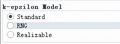
There are three k-ε models in Fluent: the standard k-ε model, the RNG k-ε model, and the Realizable k-ε model.

2.1 Standard k-ε Model
As mentioned above, a one-equation model requires the turbulence length scale l to be specified manually. The length scale reflects the size of eddies and directly affects the mixing capability of turbulence. In a one-equation model, l often needs to be given through algebraic empirical formulas:
- Very near-wall region: l \sim y^2
- Moderately near-wall region: l \approx ky (k = 0.4 \sim 0.41)
- Region away from the wall: l \approx (0.075 \sim 0.09)\delta, where \delta is the boundary-layer thickness
- If the turbulence is a free shear flow, it is similar to the region away from the wall: l \sim b(x), where b(x) is the jet width.
Once the flow geometry becomes complex, such as with separation, recirculation, or multiple components, this length scale becomes difficult to specify accurately.
The k-ε model among two-equation models no longer requires the empirical specification of a length scale. It has a wide range of applicability and has become the mainstream in engineering.
The k-ε model still follows Boussinesq’s eddy viscosity hypothesis. The proportionality coefficient is the turbulent viscosity \mu_t, but it expresses \mu_t using the turbulent kinetic energy k and the dissipation rate \varepsilon:
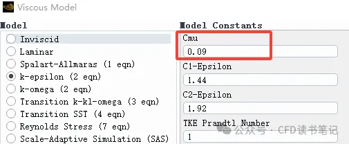
The above formula is obtained through dimensional analysis, where C_\mu is an empirical constant of about 0.09, namely the Cmu parameter in the k-epsilon turbulence model in Fluent:
This formula is highly consistent with physical intuition: the stronger the turbulence, the larger k is and the larger \mu_t is; the faster the turbulent energy dissipates, the larger \varepsilon is and the smaller \mu_t is.
Now \mu_t can be expressed, but how are k and \varepsilon calculated? The k-ε model solves k and \varepsilon through transport equations:
k equation (describes the production, diffusion, and dissipation of turbulent kinetic energy):
\varepsilon equation (describes the production, diffusion, and destruction of the dissipation rate):
The production term G_k comes from the work done by the mean velocity gradient, and the dissipation term is \rho\varepsilon. The \varepsilon equation is not derived directly; instead, it is constructed by imitating the form of the k equation and includes production, diffusion, and destruction terms. It determines the rate of turbulent dissipation, thereby indirectly controlling the evolution of the turbulence length scale.
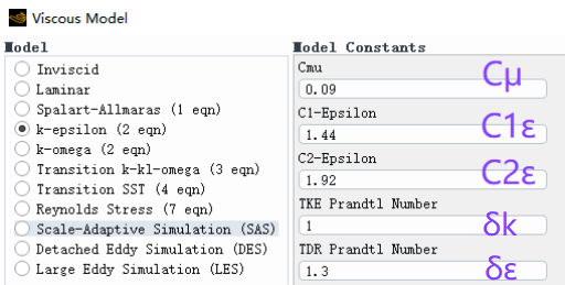
Combining \mu_t, k, and the \varepsilon equation, we can see that several constant parameters appear in the formulas: C_\mu, C_{1\varepsilon}, C_{2\varepsilon}, \sigma_k, and \sigma_\varepsilon. In 1974, Launder & Spalding gave the classic values of these parameters:
| Parameter | Value |
|---|---|
| C_\mu | 0.09 |
| C_{1\varepsilon} | 1.44 |
| C_{2\varepsilon} | 1.92 |
| \sigma_k | 1.0 |
| \sigma_\varepsilon | 1.3 |
These parameters are called classic because a large number of subsequent experiments have verified their correctness. Therefore, unless there is a very sufficient reason, these parameters generally do not need to be changed.
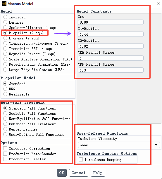
The default values of these parameters in Fluent are also the same:
The standard k-ε model is computationally stable and has good convergence. It has also been validated by a large number of experiments, and its accuracy is acceptable for flat-plate boundary layers, pipe flows, and jets. It is the first-choice RANS model in almost all CFD software.
However, it also has some shortcomings, mainly including:
- Unable to handle strong swirling flow: The isotropic eddy viscosity hypothesis fails in strongly rotating flows, and the predicted rotation effect is too weak.
- Round pipe jets spread too quickly: The predicted jet width is about 40% wider than experimental results, because the model overestimates the diffusion of turbulent viscosity at the jet center.
- Near-wall regions rely on wall functions: It needs to be used with logarithmic-law wall functions, and its accuracy decreases under strong pressure gradients or in separated regions.
It is precisely these defects that led to two famous improved versions of the standard k-ε model: RNG k-ε and Realizable k-ε.
2.2 RNG k-ε Model
RNG = Renormalization Group, a statistical theoretical method. In 1986, Yakhot & Orzag used mathematical derivation to modify the \varepsilon equation and obtained RNG k-ε.
An additional source term R_\varepsilon is added to the \varepsilon equation:
The newly added term R_\varepsilon is:
where:
The constants are \eta_0 = 4.38 and \beta = 0.012.
If we combine the R_\varepsilon and C_{2\varepsilon} terms in the equation, the \varepsilon equation can be written as:
This form is the same as the form of the \varepsilon equation in the standard k-ε model, but the key difference is that C_{2\varepsilon}^* is no longer a constant.
The benefit of this is that in regions with high strain rate, that is, large \eta, such as strong swirling flow or wall curvature, C_{2\varepsilon}^* automatically increases. This enhances the destruction term in the \varepsilon equation, causing the turbulence dissipation rate \varepsilon to be “pushed up”, which lowers the turbulent viscosity \mu_t, weakens excessive turbulent mixing, and improves the prediction of swirling flow and separation.
In low-strain-rate regions, \eta tends toward 0, and R_\varepsilon also tends toward 0. At this point, the RNG model becomes the standard k-ε model.
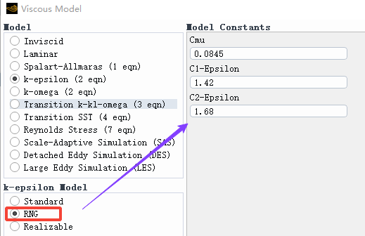
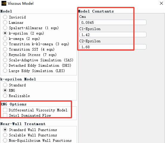
Therefore, we can see that the RNG model extends the standard model, making the standard model more accurate in predicting high-strain-rate flows. At the same time, the constant values of the RNG model also differ from those of the standard model. Theoretically, C_\mu \approx 0.0845 is calculated, and the other parameter values are C_{1\varepsilon} = 1.42 and C_{2\varepsilon} = 1.68.
In Fluent, the RNG model usually uses the effective viscosity ratio to interpolate \sigma_k and \sigma_\varepsilon instead of using fixed values, so these two parameters are not available in the interface:
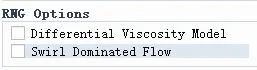
In addition to the above parameter settings, the RNG model also has two accompanying options. We will explain this part in detail in the interface introduction in Section 3.

To summarize, the RNG k-ε model is sensitive to strong strain rates and is more accurate for separated flows and rotating flows. It is suitable for flows such as jets and cyclone separators. However, in essence, it is still a turbulence model for high Reynolds numbers and consumes about 10%–15% more CPU time.
2.3 Realizable k-ε Model
Previously, we introduced the standard k-ε model and the RNG k-ε model. The standard k-ε model sets 5 constant parameters, while the RNG k-ε model expresses C_{2\varepsilon} among the constant parameters as an equation related to strain rate, making the model more suitable for strong-strain-rate flows.
Both models assume that C_\mu is a constant. This assumption works well in flat-plate boundary layers and round pipe flows, but problems arise when strong strain rates or large-curvature flows are encountered.
The most classic example is a round pipe jet. Experiments have found that the turbulent viscosity in the jet core region should be far lower than the prediction of the standard model, causing the jet spreading rate to be about 40% faster than the experimental value. Why does the standard model overestimate \mu_t?
Because k^2/\varepsilon is calculated to be too large at the jet center, while C_\mu is locked at 0.09, resulting in excessive turbulent viscosity. From a physical perspective, Reynolds stresses must also satisfy certain physical constraints.
Therefore, to achieve this goal, Shih et al. proposed the Realizable k-ε model in 1995. Its core objective is to make C_\mu no longer a constant, but instead dynamically adjusted with the mean flow field, and to accurately predict jet spreading.
The expression for C_\mu in the Realizable model is:
where:
S_{ij} is the mean strain-rate tensor, and \Omega_{ij} is the mean rotation-rate tensor (taking angular velocity into account).
When the mean strain rate S is large, U^* becomes larger, and the A_s U^* k/\varepsilon term in the denominator dominates. C_\mu automatically decreases, and the turbulent viscosity decreases accordingly. This achieves a limiting effect on the turbulence prediction.
At the same time, the Realizable model also improves the \varepsilon equation. The \varepsilon equation of the standard model comes from empirical derivation rather than strict theoretical derivation.
The Realizable model derives the \varepsilon equation starting from the transport equation:
- Production term: \rho C_1 S \varepsilon. Compared with the standard \varepsilon equation, it directly uses S multiplied by \varepsilon, avoiding singular behavior caused by k in the denominator.
- Destruction term: \sqrt{\nu\varepsilon} is added to the denominator, ensuring that it does not diverge in the near-wall region.
To summarize, the Realizable k-ε model re-derives C_\mu and the \varepsilon equation, allowing the Reynolds stresses to satisfy physically realizable conditions. Therefore, it is usually the best choice for rotating homogeneous shear flows, free flows containing jets and mixing flows, internal pipe flows, boundary-layer flows, and flows with separation.
The Fluent Theory Guide specifically points out that the Realizable model can more accurately predict the spreading rate of jets.
2.4 Comparison of the Three k-ε Models
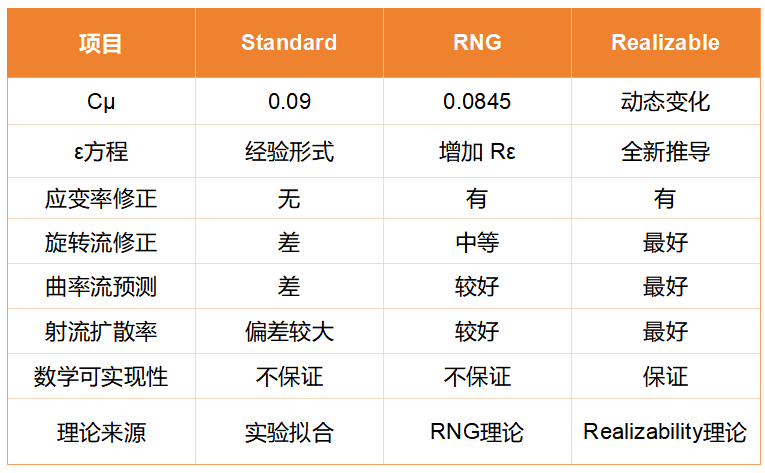
We use AI to summarize and generate a comparison table of the three models:
3. Fluent k-ε Model Interface
3.1 Standard k-ε Model Interface
Here we only discuss the additional parameter settings for each turbulence model. The general parameters will not be mentioned for now.
For the standard k-ε model, what needs to be set is the group of constant parameters at the upper right of the interface, namely the parameters given in Section 2.1:
C_\mu=0.09, C_{1\varepsilon}=1.44, C_{2\varepsilon}=1.92, \sigma_k=1.0, \sigma_\varepsilon=1.3
These constants have undergone extensive engineering validation and generally do not need to be modified. Or, to put it another way, if you want to modify these parameters, you need to provide a reason that can convince others.
3.2 RNG k-ε Model Interface
The RNG k-ε model interface also requires some constant parameters to be set, which have already been introduced in Section 2.2. Below, we focus on the settings for RNG Options:
Differential Viscosity Model: Selecting this option means using the differential formula for effective viscosity \mu_{eff} to account for low-Reynolds-number effects:
where \hat{\nu} = \mu_{eff}/\mu, representing the ratio of effective viscosity to molecular viscosity.
This differential equation can better describe the transition from the viscous sublayer to the logarithmic-law region. It can be used to select the low-Reynolds-number RNG mode and integrate directly to the wall without relying on wall functions.
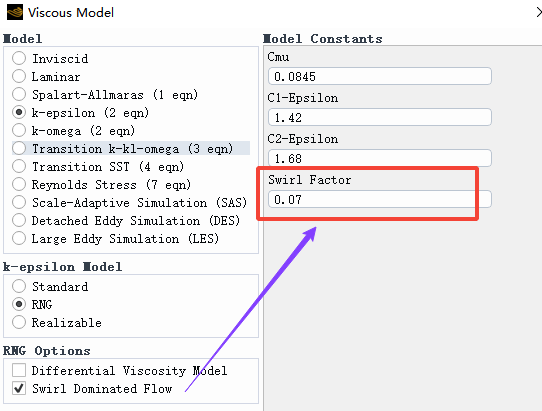
Swirl Dominated Flow: For the RNG model, swirl correction can be enabled in strong swirling flows. At this point, the turbulent viscosity \mu_t is multiplied by a function related to the swirl number:
At this point, an additional parameter setting appears in the interface:
Fluent provides the swirl constant \alpha_s, with a default value of 0.07. For strong swirling flow, it can be increased to around 0.1 to further suppress excessively high turbulent viscosity.
3.3 Realizable k-ε Model
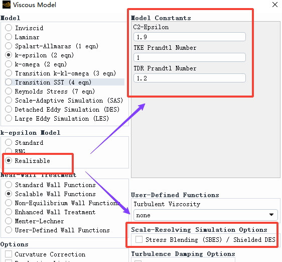
The Realizable k-ε model requires some constant parameters to be set, which can generally be kept at their default values:
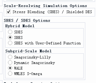
In addition to constant parameters, the Realizable k-ε model can also enable the SBES or SDES model, that is, by selecting Stress Blending (SBES) / Shielded DES.
After selecting this option, the settings become relatively complex. Here, we only explain the purpose of this option and will not introduce it in detail:
After selecting this option, it is equivalent to embedding LES functionality into the RANS governing equations. It is a hybrid RANS-LES method. RANS is used to handle attached boundary layers, while LES captures large-scale separated eddies away from the wall.