Fluid-Structure Interaction (FSI) refers to the process of mutual interaction and influence between fluid flow and solid structures:
The fluid transmits its pressure and thermal loads to the solid.
When the solid is subjected to gas pressure or thermal loads, it undergoes deformation. If this deformation is significant enough to affect the flow field, a two-way FSI approach is required.
If the solid’s deformation is minor, the reverse impact on the fluid can be neglected, leading to a one-way FSI approach.
The solid may also experience deformation due to other external forces, which can further influence fluid flow.
If the solid undergoes significant deformation due to external forces affecting fluid flow, a two-way FSI analysis is also necessary.
Why Conduct Fluid-Structure Interaction Analysis?
Many complex unsteady problems involve interactions between fluids and solids. Only by using a two-way FSI analysis can the true nature of physical phenomena be captured.
Analysis Strategy
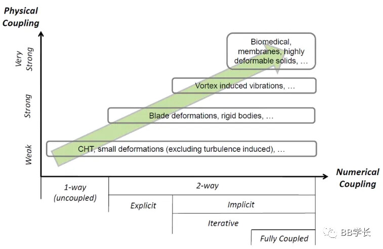
FSI analysis can be classified based on the degree of interaction between physical phenomena:
A higher degree of coupling between different physical fields necessitates a two-way coupling approach.
In cases of weaker coupling between different physical fields, a one-way coupling solution method can be employed.
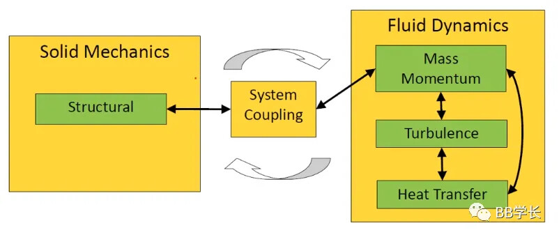
The data transferred between MAPDL and CFD requires multiple steps of coupling iterations to achieve convergence. This is similar to the iterative solving needed in both CFD and FEA to obtain convergent computational results.
The following parameters can be transferred:
Aerodynamic Forces
Geometric Deformation
Temperature
Heat Flux
Heat Transfer Coefficient and Reference Temperature for Heat Transfer Coefficient
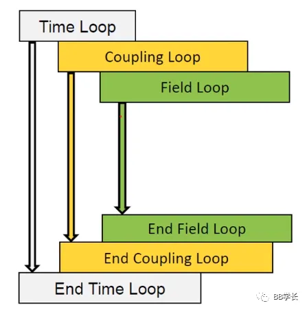
The Field Loop stops iterating once convergence is achieved in a single physics field (or after reaching the maximum number of iterations).
CFD does not need to converge at every coupling step; it only needs to converge in the last coupling step of a time step.
The Coupling Loop stops iterating once the transmitted data at the coupling interface converges (or after reaching the maximum number of iterations).
Ensure that each individual flow field and the transmitted data converge before proceeding to the next time step.
Example Calculation:
If Fluent’s Field Loop iteration count is 10, Coupling Loop iteration count is 5, and the total number of time steps is 100, then the total maximum computational steps for Fluent would be:
10×5×100=500010 \times 5 \times 100 = 500010×5×100=5000.
Coupling Simulation Types: Based on Fluent and Mechanical, both steady-state and transient one-way/two-way coupling simulations are available.
Data Transfer: Aerodynamic forces and geometric deformations are transferred between Fluent and Mechanical.
Heat Transfer: Heat flux and heat transfer coefficients are exchanged between Fluent and Mechanical.
Iterative Calculations: The coupled simulation performs iterative calculations to achieve implicit computational results.
Element Compatibility: All result elements are applicable, including SOLID, SHELL, and SOLSH elements; most features of Fluent are supported.
Continuity of Calculations: Supports continuation of calculations after stopping; post-processing can be performed in CFX-Post; parameterization is supported.
Overview of the Operation Process
Fully Transient Two-Way Fluid-Structure Interaction Simulation: This allows for the transmission of deformations, aerodynamic loads, and thermal loads between fluids and solids.
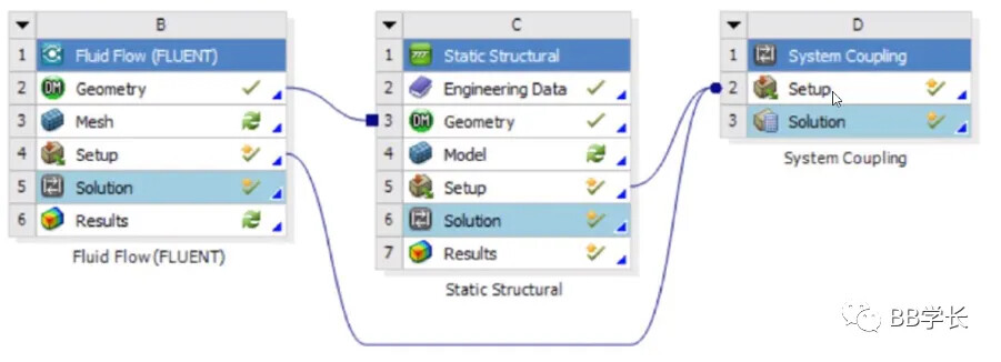
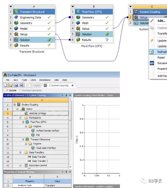
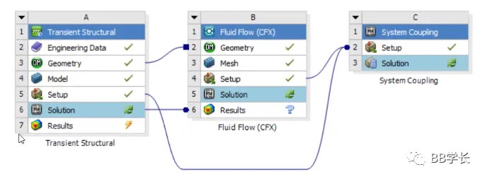
Workbench Standard Workflow: Workbench provides a standard workflow for fluid-structure interaction analysis.
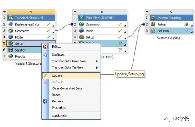
Setup Connections: Connect the Fluent setup unit and Static/Transient/Thermal setup to the System Coupling setup.
After the calculations are completed, you can call the separate Result Post tool for displaying the results.
Drag Solution to View Combined Results:
Alternatively, you can drag the Solution unit from Transient/Thermal into the Results section of Fluent to view both fluid and solid computational results together.
Introduction: Setting Up Fluent and Mechanical for Fluid-Structure Interaction (FSI)
Setup Settings in Mechanical
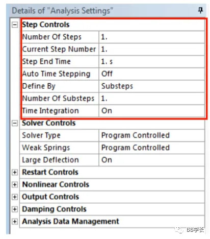
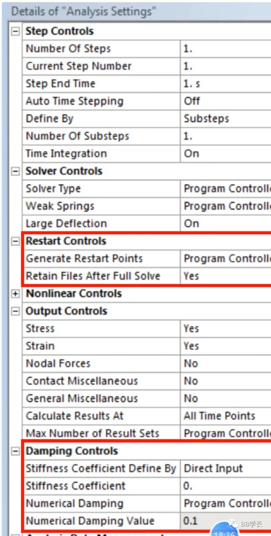
Number of Steps:
Set Number of Steps to 1. The Step End Time must not be less than the required computation time.
Load Application:
Only single-step load applications are allowed. You can change the load by restarting the computation or use a Table data list to simulate time-varying loads.
Time Duration:
The Time Duration is controlled by System Coupling (SC) but must not exceed the Step End Time.
Auto Time Stepping:
Set Auto Time Stepping to Off.
Choose Define By as Substeps and set Number of Substeps to 1.
Time Step Considerations:
If the time step size in MAPDL is smaller than that in Fluent, you can select Auto Time Stepping or Multiple Substeps. The entire time step will be based on the settings in SC.
Caution with Define By:
Be cautious when setting Define By to Time; the time step size configured in SC will be adopted by MAPDL.
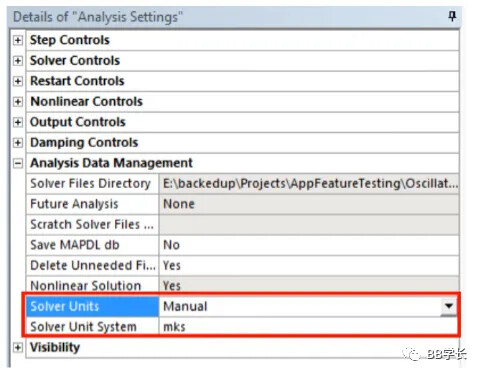
Set Solver Unit System to mks (meters, kilograms, seconds). This setting will replace the unit system in Workbench and Mechanical with the selected unit system.
Recommendation:
It is recommended that users adopt this setting, as in many cases, users may not be aware of the default unit system used by other installations of ANSYS software.
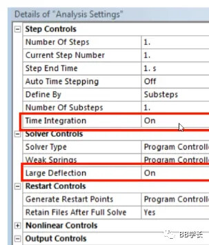
Set to On: This option allows for the consideration of unsteady effects (such as inertia).
Alternatively, you can set it to Off to generate steady-state results, which can be used to produce initialization results. However, Fluent should still be set to perform transient calculations.
Large Deflection:
Generally, this option should be set to On.
If set to Off, the mesh will not deform during the calculation, and the loads throughout the coupling process will act on the initial mesh only.
Set Solver Unit System to mks (meters, kilograms, seconds). This setting will replace the unit system in Workbench and Mechanical with the selected unit system.
Recommendation:
It is recommended that users adopt this setting, as in many cases, users may not be aware of the default unit system used by other installations of ANSYS software.
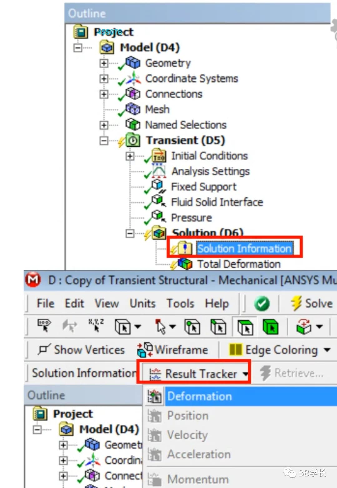
Navigate to Result Tracker and select Deformation.
Node Selection:
In the geometry structure, select a node, or choose a mesh node from the toolbar.
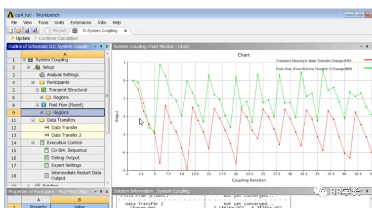
Chart Generation:
After the calculations are completed, a chart will be automatically generated. The System Coupling (SC) will update and display the monitored data changes throughout the solving process.
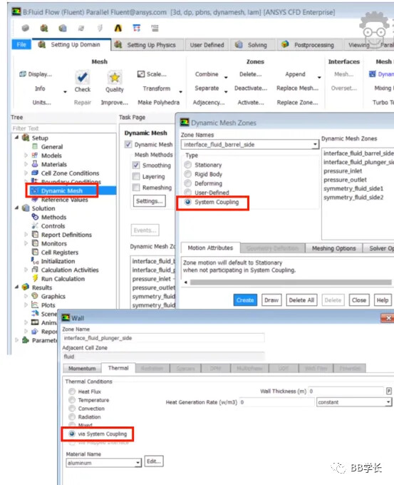
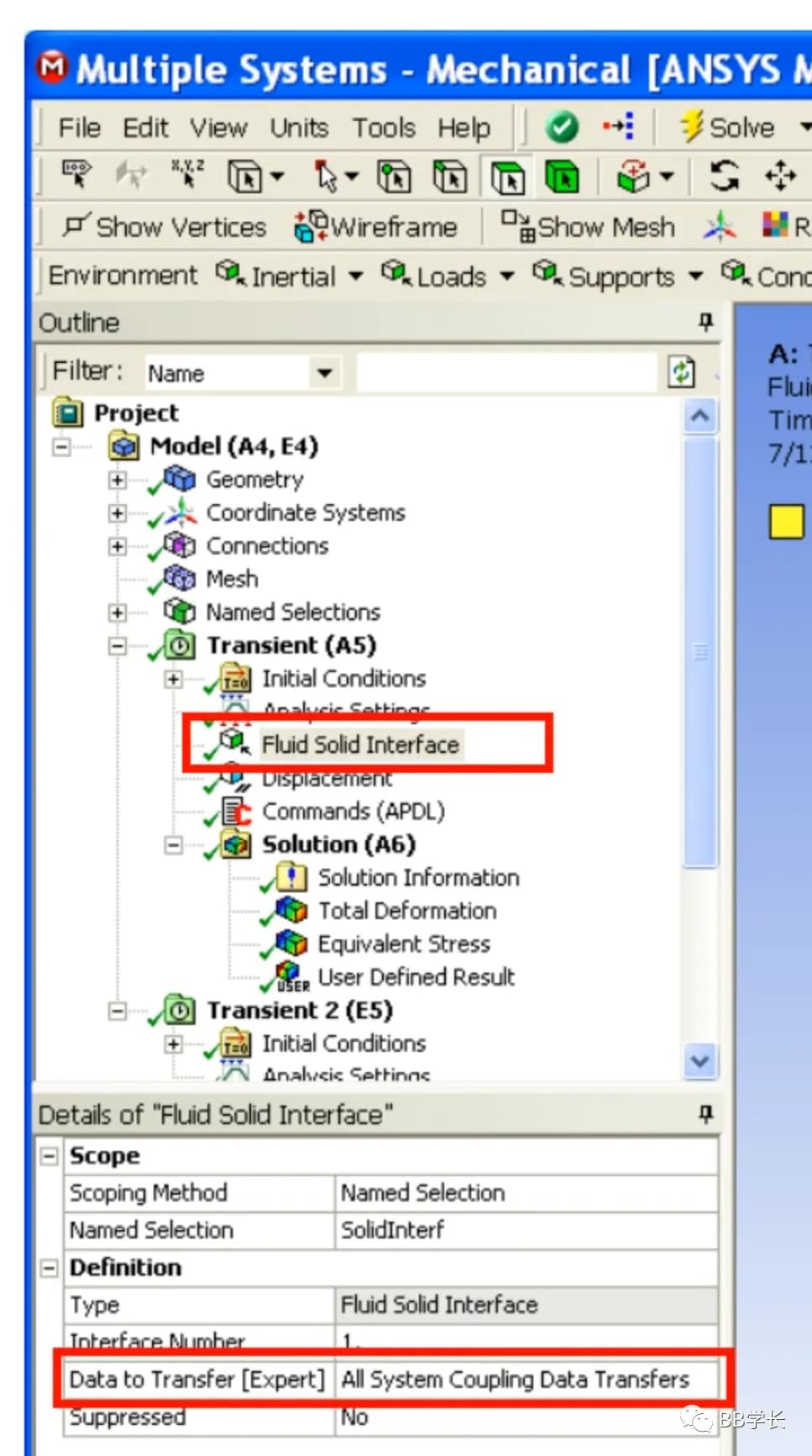
Set Data to Transfer [Expert] to All System Coupling Data Transfers.
This configuration enables the transfer of thermal data on the coupling interface.
Command Line Addition:
Add necessary command lines to activate the coupling field elements.
Ensure to set the structural thermal boundary conditions appropriately.
Boundary Conditions:
Define the thermal boundary conditions for the structure to facilitate accurate data transfer during the coupling process.
By configuring these settings, both structural and thermal data can be effectively transmitted across the coupling interface, allowing for a comprehensive analysis of the interactions between the solid and fluid domains.
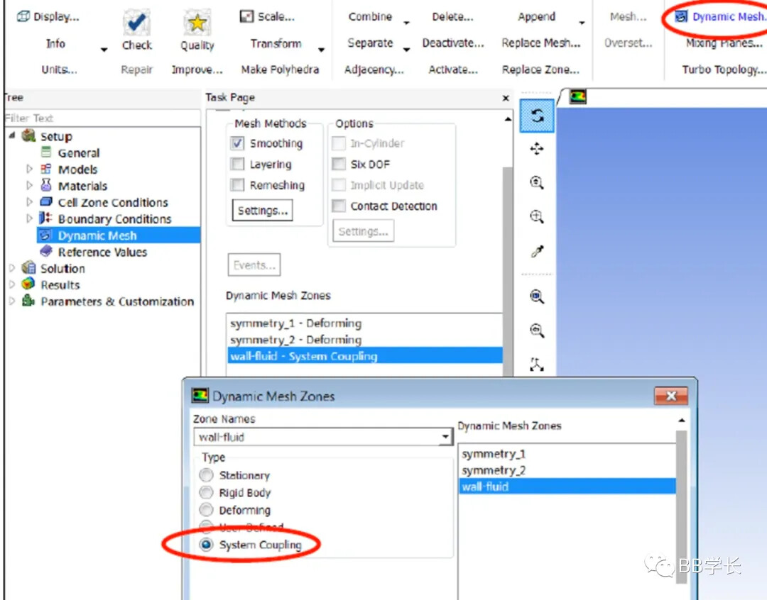
Select Dynamic Mesh and set the Dynamic Mesh region to the System Coupling option.
Ensure that the surfaces in the System Coupling region are configured to accept deformation transfer.
Default Regions:
By default, all regions are set as stationary regions unless specified otherwise.
These configurations ensure that the fluid domain is capable of interacting dynamically with the structural changes from the solid domain during the coupling analysis.
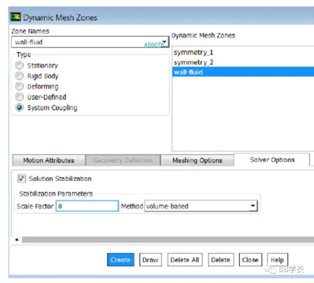
For the dynamic mesh region at the System Coupling interface, you can enable Solution Stabilization on the Solver Options page.
Purpose of Solution Stabilization:
This parameter enhances the robustness of force and deformation transfer during strongly coupled calculations, helping to prevent computational divergence.
Enabling solution stabilization is particularly important in scenarios where significant interactions between the fluid and solid domains occur, ensuring a more stable and reliable analysis outcome.
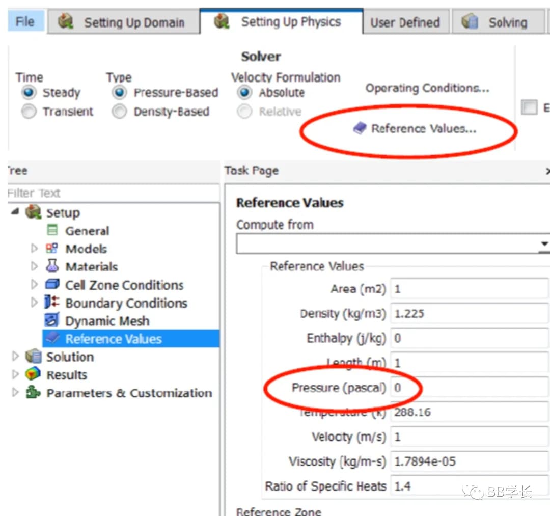
In the Setting Up Physics section, you can set the reference pressure to 0.
Additional Reference Values:
You can also set other reference values such as size, density, etc., for subsequent non-dimensional parameter analysis.
Impact of Reference Pressure:
When the reference pressure is set to 0, the aerodynamic forces will correspond to absolute pressure. If a different value is set, the pressures transferred will be relative pressures.
Setting appropriate reference values is crucial for accurate results, particularly in fluid dynamics simulations where pressure differentials are significant.
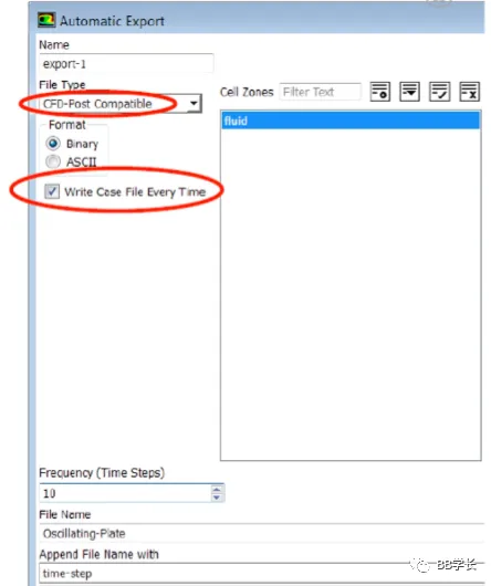
Typically, the output result settings in Fluent can be left at their default configurations.
Automatic Export:
You can modify the output format and output intervals under the Automatic Export section to suit your needs.
Adjusting these settings allows you to control how frequently results are exported and in what format, ensuring that you receive the necessary data for analysis.
Physical Property Parameter Settings for Compressible and Incompressible Fluids
Density Settings:
For both compressible and incompressible fluids, it is advisable not to set the fluid density as a constant. Instead, density should be treated as a variable that can change with temperature.
Ideal Gas Model:
For low-speed and high-speed gases, it is recommended to set them as ideal gases, meaning the density will be a function of temperature changes. This approach captures the behavior of gases more accurately across different operating conditions.
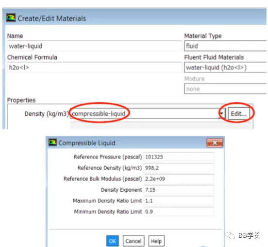
Compressible Liquid Model:
For liquids, it is also beneficial to treat them as compressible fluids, even if the density changes with temperature and pressure are minimal. This setting can significantly aid in achieving convergence in the numerical solution.
By properly configuring the physical properties of the fluids in your simulations, you enhance the accuracy of the results and improve the convergence behavior of the computational model.
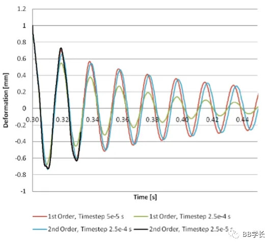
The default setting is the 1st-order implicit solver. However, it is recommended to use the 2nd-order implicit format for solving transient problems.
Time Step Considerations:
Utilizing a 2nd-order implicit format may require smaller time step sizes to achieve convergent results. This adjustment helps ensure the accuracy and stability of the simulation, especially in transient analyses where rapid changes in conditions occur.
By choosing the appropriate solver format and managing the time step size, you can improve the convergence and reliability of the transient analysis in your simulations.
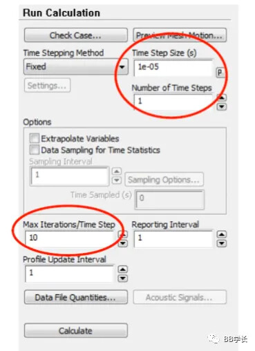
The Time Step Size and the Number of Time Steps are controlled by parameters in the System Coupling interface.
Maximum Iteration Steps per Time Step:
The maximum number of iterations allowed within each time step should not be too high. The default value is 20, but it is generally recommended to change this to 10.
This adjustment helps optimize the computational process, ensuring that each time step converges effectively while preventing excessive computational load.
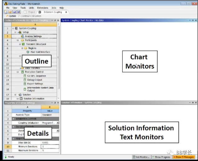
The Operation Interface is Divided into Four Sections:
Operation Tree:
This section provides a hierarchical view of the various components and settings of the simulation. Users can navigate through the different modules and configurations.
Monitoring Curve Display:
Here, the monitoring curves are displayed in real-time, allowing users to observe the convergence behavior and key performance indicators throughout the simulation process.
Detailed Settings Information:
This area presents detailed information about the selected settings, enabling users to modify and fine-tune parameters for better control over the simulation.
Log Information Display:
This section shows the logs and messages generated during the simulation, providing insights into the progress, warnings, or errors encountered.
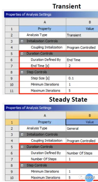
In the System Coupling (SC) interface, the duration of the analysis for both the structure and fluid is controlled uniformly. This ensures that the time lengths are synchronized across the coupled analysis.
Setup Control:
For Transient Analysis:
Time steps and iteration counts for data exchange between the structure and fluid can be set here. This allows for a defined structure and fluid time step length, as well as the number of iterations for data exchange between the two domains.
For Steady-State Analysis:
This section allows you to set the iteration counts for data exchange between the structure and fluid, ensuring that the necessary interactions are accurately captured during the steady-state analysis.
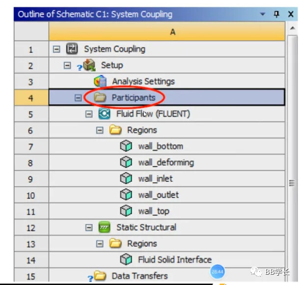
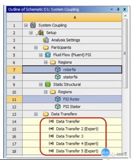
In the System Coupling (SC) interface, the Participants section displays the various coupling interfaces between the structure and fluid.
Fluent Interfaces:
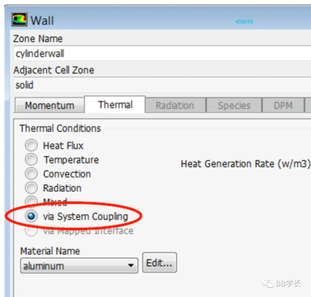
Each wall surface in Fluent will be listed, allowing you to designate them as fluid-solid coupling interfaces. This facilitates subsequent matching of these interfaces.
Ordinary wall surfaces can unidirectionally transfer aerodynamic forces and heat transfer data to the structural calculation elements.
Mechanical Interfaces:
The Fluid-Solid Interaction (FSI) interfaces from Mechanical will also be displayed, ensuring that all relevant interfaces for the coupling are accounted for in the simulation.
These settings are crucial for establishing the correct interactions between the fluid and structural domains, enabling accurate data transfer and ensuring the integrity of the coupled simulation process.
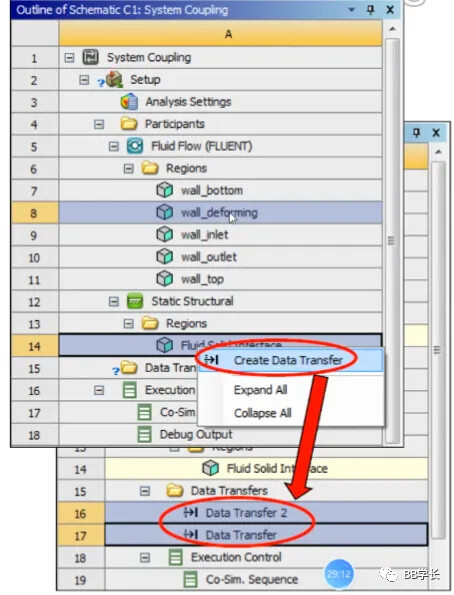
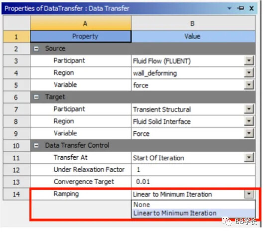
Once a set of fluid-structure interaction (FSI) interfaces is created, it will include two Data Transfer entries: one for transferring forces to the structural elements and another for transferring deformations to the fluid elements.
For thermal-fluid coupling interfaces, three Data Transfer entries will be included: temperature, heat transfer coefficient, and near-wall temperature.
In the case of thermal-fluid-structure coupling interfaces, all five of the aforementioned Data Transfer entries will be included.
None: All transferred data is loaded in a single iteration exchange step during the first iteration.
Linear to Minimum Iteration: Throughout the entire time step, the load data is gradually applied in a linear manner, controlled by the Minimum Iteration number.
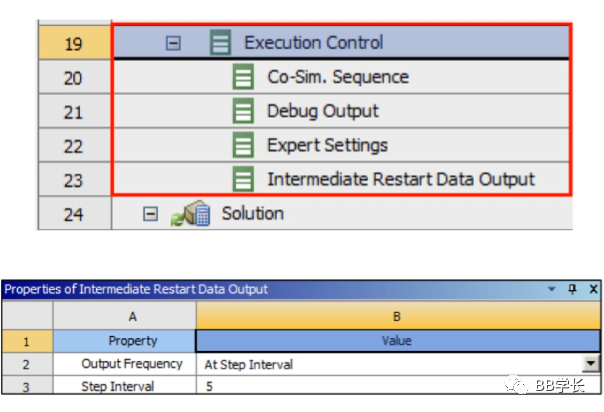
Intermediate Restart Data Output: This setting controls the interval for saving intermediate process files, which can be used to restart the calculation after an interruption.
For fluid-structure interaction (FSI) calculations, the settings in the Mechanical Analysis Setting are largely consistent with those of general computations, requiring no major modifications for different problems.
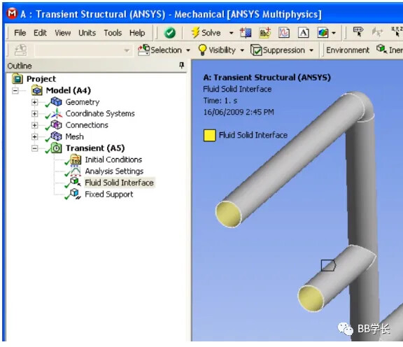
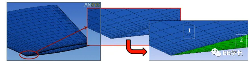
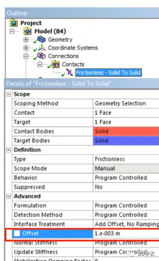
Fluid Solid Interface: In Mechanical, set the surfaces that need to transfer deformation as Fluid Solid Interfaces for subsequent data transfer.
Dynamic Mesh in Fluent: In Fluent, enable the Dynamic Mesh setting and activate the System Coupling option to select the coupling interfaces for data transfer.
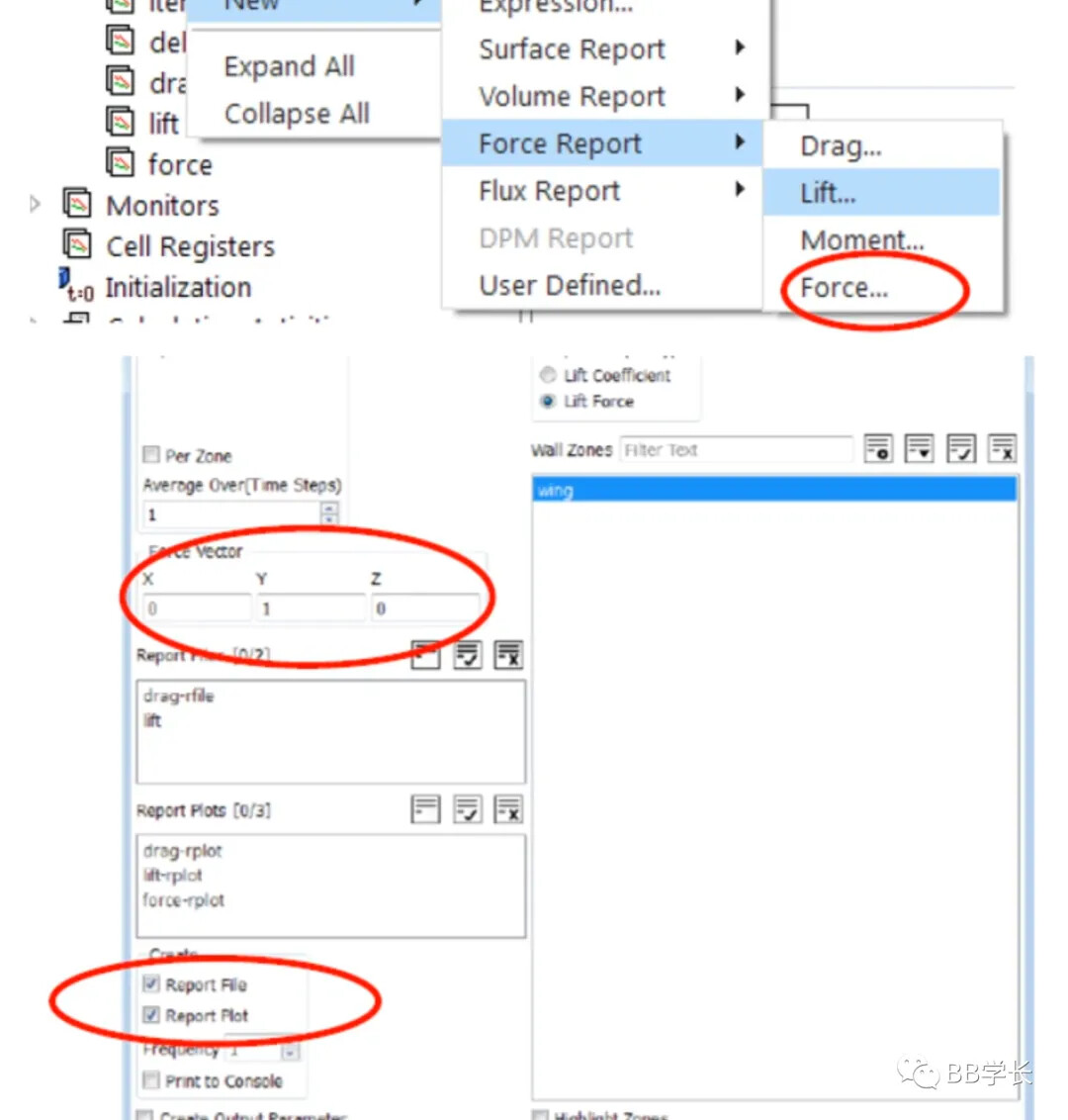
Monitoring Points: Create monitoring points for forces and heat exchange data on the coupling interfaces in Fluent.
Solution Trackers: In Mechanical, use Solution Trackers to monitor the deformation at specific points.
System Coupling Setup: In the System Coupling interface, create data exchange interfaces, calculation steps, and time step sizes; set the interval for saving calculation files to prevent interruption of computations.