Note:
All files required for this article, including Python code, UDF code, CAS and DAT files, and GIF image files, are provided in the link at the end of the article.
1. Cloud Plot Emoji Pack Description
This cloud plot emoji pack has certain limitations, specifically, it is only applicable to black and white line-based emoji packs. In the cloud plot, red represents black and blue represents white. This is because the cloud plot color varies from blue to red, while the emoji pack color may cover the entire RGB range. I am not sure how to display RGB colors in the cloud plot.
Of course, I tried directly adding RGB colors, and it did result in a color cloud plot, but the result looked like a thermal imaging photo.

2. Cloud Plot Emoji Pack Generation Approach
There are several ways to generate this cloud plot, and the use of profile files can also achieve some of the effects. However, the simplest implementation is still using Python combined with UDF.
Approach and Steps: We know that animated images are created by stacking many frames, and the cloud plot emoji pack follows the same principle.
2.1 Obtaining the Key Frames of the Emoji Pack
First, we need to obtain the key frames of the emoji pack. This can be done using the WPS image editor.
Use the WPS image editor to convert the emoji GIF file into many images.
2.2 Python Pixel Recognition
This step is done using Python. The Python script converts the emoji pack’s image files into pixel data and writes the pixel data for each image into a TXT file.
For example, if an emoji GIF image produces 20 PNG images, Python can generate 20 profile files. Each profile represents the pixel data of one image.
2.3 UDF Dynamic Import of Pixel Data
Now that we have obtained the pixel data of the image, we need to import this data into Fluent. How to import it? There are two ways: profile files and UDF. However, UDF is simpler and more streamlined.
To achieve the animation effect, we need to import a profile at each iteration step and force the temperature or other variables to change according to the pixel data. Each iteration step draws one frame, and 20 frames make 20 iterations, connecting them together will create the animation effect.
2.4 Fluent Animation Creation
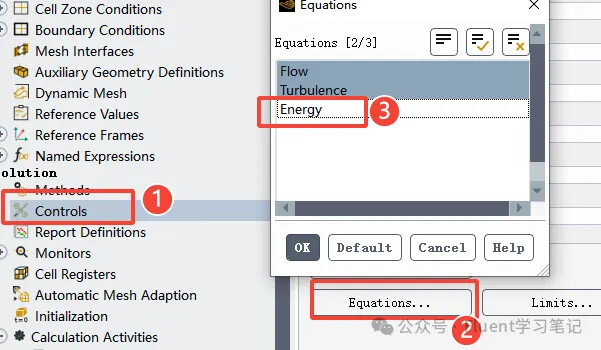
This is the standard process of generating animations in Fluent. Before generating the animation, make sure to check the energy equation, and then uncheck the energy equation in the control settings.
The purpose of this step is to prevent Fluent’s default solver from interfering with the generated images.
3. Emoji Pack Case Example
The above describes the overall approach and steps. Now let’s go through an example to explain in more detail.
3.1 Obtaining the Key Frames of the Emoji Pack
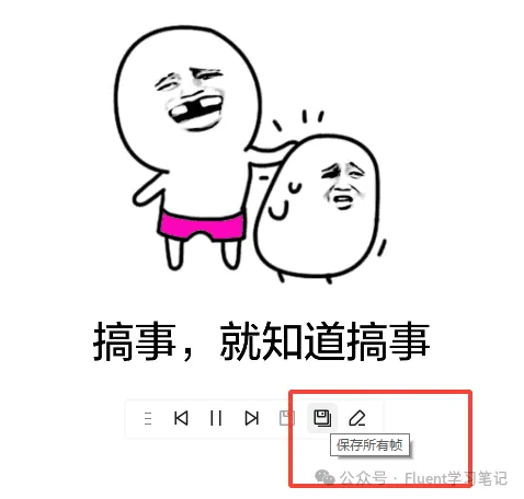
First, search for the emoji pack and save it.

Open the emoji GIF with WPS and click “Save All Frames.”
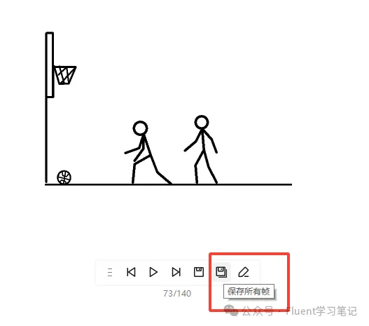
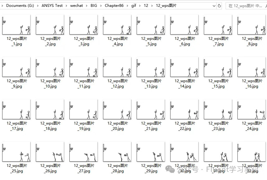
You can find the folder with all the frames of the emoji in the folder where the emoji images are saved. These are the source images for generating the cloud plot animation.
3.2 Python Pixel Recognition
Basic Logic: Python reads the image pixels, and if the pixel color is below a certain threshold, it records the coordinates of that pixel; otherwise, it skips it.
Here is the complete Python code:
from PIL import Image
import matplotlib.pyplot as plt
def get_coordinate(path):
# Open image
image = Image.open(path)
width, height = image.size
length_x = 4 # Model size in Fluent, x-direction, adjust according to cloud plot emoji pack size
length_y = 3 # Model size in Fluent, y-direction, adjust according to cloud plot emoji pack size
x_list = [] # x coordinates
y_list = [] # y coordinates
out = image.convert("RGB")
num = 0
for i in range(width):
for j in range(height):
num += 1
if (out.getpixel((i, j)) < (50, 50, 50)): # RGB value less than the threshold, larger value captures more pixels
x = i / width * length_x
y = (height - j) / height * length_y
if (num % 2 == 0): # Skip some data
x_list.append(x)
y_list.append(y)
return x_list, y_list
def write_file(x_list, y_list, path, UDF=0, draw=1): # Open file to write, create it if it doesn't exist
if(UDF == 1): # If using UDF, UDF=1, generate the txt data for UDF, otherwise generate profile files
with open(path, 'w') as file:
for i, x in enumerate(x_list):
file.write("{:.5f} {:.5f}\n".format(x, y_list[i]))
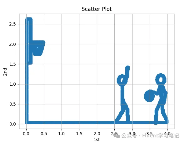
if(draw == 1): # Whether to display the image, 1 means display
plt.scatter(x_list, y_list, marker='o')
plt.grid(True)
plt.xlabel('1st')
plt.ylabel('2nd')
plt.title('Scatter Plot')
plt.show()
if __name__ == '__main__':
"""---------------------------- System Animation ------------------------"""
MAX_DATA_POINTS = []
for i in range(1, 141): # 141 represents the number of frames, adjust as needed
path = r"G:\ANSYS Test\wechat\BIG\Chapter94\gif\12\12\\" + "12_wps_image_{:d}.jpg".format(i) # Frame image address, change according to your needs
x_list, y_list = get_coordinate(path)
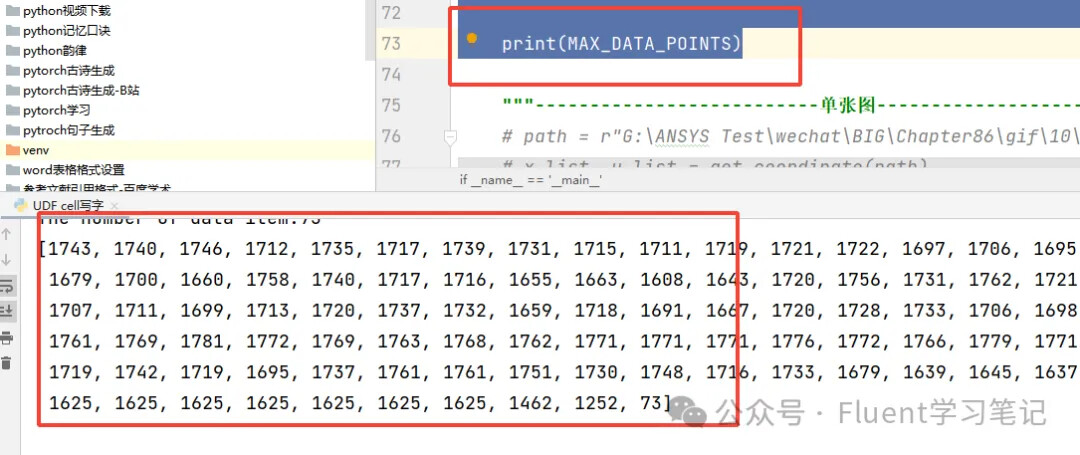
print("The number of data items: {:d}".format(len(x_list)))
MAX_DATA_POINTS.append(len(x_list))
path1 = r"G:\ANSYS Test\wechat\BIG\Chapter94\gif\12\12\\" + "{:d}.txt".format(i) # UDF file address, change according to your needs
if i % 50 == 0: # Draw a plot every 50 frames
draw = 1
else:
draw = 0
write_file(x_list, y_list, path1, UDF=1, draw=draw)
print(MAX_DATA_POINTS)
It can be divided into four main steps: image processing, coordinate extraction, data export, and visualization. The overall process is as follows:
a. Image Processing and Opening
The code loads the image frame by frame from the specified image path. It uses the PIL.Image.open function to open the image and convert it to RGB format.
b. Coordinate Extraction
The code traverses each pixel of the image and extracts the darker pixels (those with RGB values below the set threshold, (50, 50, 50)).
c. Data Export
After processing each frame of the image, the extracted coordinate data can be saved in UDF format. If UDF=1, the coordinates are saved as text, which will be used for Fluent’s custom user-defined function (UDF).
d. Visualization
Every 50 frames, the code, based on the parameter draw=1, calls matplotlib.pyplot to draw and display a scatter plot of the extracted coordinate data, which is helpful for visual verification.
e. Main Program Control Flow
The main function processes 141 frames of images, and each frame calls the get_coordinate function to extract the coordinates and then calls write_file to save the data.
The image frame address and output file path are dynamically generated based on the image number, and each frame’s UDF data is saved as a .txt file.
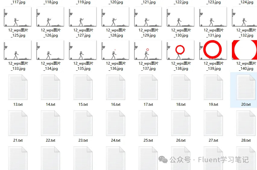
After completing the above steps, a large number of pixel coordinate TXT files are generated, one for each image. These files are the ones that UDF will need to read.
Adjust the following code lines: 8, 9, 17, 20, 43, 44, 48, 49.
3.3 UDF Dynamic Import of Pixel Data
Now, UDF will read these TXT files.
Basic logic: Each iteration step reads a TXT file and loops through the entire computational domain grid, checking if the coordinates in the TXT file match the current grid coordinates. If they match, the temperature is changed. The next iteration step will read the next TXT file.
Here is the complete UDF code:
#include "udf.h"
#include <stdio.h>
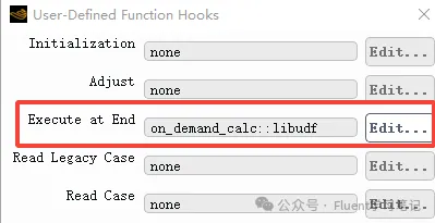
DEFINE_EXECUTE_AT_END(on_demand_calc)
{
cell_t c;
Domain *d;
Thread *t;
d = Get_Domain(1);
real xc[ND_ND];
int j = 0;
int i = 0;
// Number of data points in each file, modify based on actual situation
int MAX_DATA_POINTS[140] = { 0, 0, 0, 0, 0, 0, 0, 0, 0, 0, 0, 0, 0, 0, 0, 0, 0, 0, 0, 0, 0, 0, 0, 0, 0, 0, 0, 0, 0, 0, 0, 3002, 4466, 6010, 7999, 8949, 10528, 11381, 11364, 11769, 11775, 11792, 11767, 11775, 11767, 11767, 11767, 11767, 11767, 11767, 11767, 11767, 11767, 11767, 11767, 11767, 11767, 11767, 11767, 11767, 11767, 12440, 14092, 15473, 17368, 18150, 20611, 21697, 23227, 23785, 24214, 24214, 24203, 24206, 24214, 24216, 24216, 24216, 24216, 24216, 24216, 24216, 24216, 24216, 24216, 24216, 24431, 26627, 28899, 30957, 31855, 33930, 35290, 36923, 38362, 40050, 40983, 42576, 43869, 45743, 46371, 46594, 46771, 46754, 46771, 46754, 46754, 46754, 46754, 46754, 46754, 46754, 46754, 46754, 46754, 46754, 46754, 46754, 46754, 46754, 46754, 46754, 46754, 46754, 46754, 46754, 46754, 46754, 48170, 49763, 51614, 52923, 54112, 55552, 57157, 58301, 58559, 58550, 58559, 58559, 58559, 58559, 58559, 58559, 58559, 58559, 58559, 58559, 58559, 58559, 58559, 58559, 58559, 58559, 58559, 58559, 58559, 58559 };
real *data_x = NULL;
real *data_y = NULL;
// Dynamic memory allocation
data_x = (real*)malloc(sizeof(real) * MAX_DATA_POINTS[N_ITER-1]);
data_y = (real*)malloc(sizeof(real) * MAX_DATA_POINTS[N_ITER-1]);
char filename[] = "G:/ANSYS Test/wechat/BIG/Chapter94/gif/12/12/"; // Data points txt file
char index[20];
sprintf(index, "%d", N_ITER); // Convert int to string
strcat(filename, index); // String concatenation
strcat(filename, ".txt"); // String concatenation
FILE *fp = NULL;
fp = fopen(filename, "r");
if (fp == NULL)
{
Message("Error: Cannot open file %s\n", filename); // Output message if the file fails to open
return;
}
else
{
Message("Successfully opened file %s %d \n", filename, N_ITER); // Output file name if successfully opened
}
while ((fscanf(fp, "%lf %lf", &data_x[i], &data_y[i]) != EOF && i < MAX_DATA_POINTS[N_ITER-1])) // Read data
{
//Message("Value %d: %lf %lf\n", i + 1, data_x[i], data_y[i]);
i++;
}
fclose(fp);
thread_loop_c(t, d)
{
begin_c_loop(c, t)
{
C_T(c, t) = 100;
C_CENTROID(xc, c, t);
for (j = 0; j < MAX_DATA_POINTS[N_ITER-1]; j++) // Loop through one set of data
{
if (((xc[0] - data_x[j])*(xc[0] - data_x[j]) + (xc[1] - data_y[j])*(xc[1] - data_y[j])) < 0.0001) // Check if position matches, the smaller the value, the finer the plot
{
C_T(c, t) = 1000; // If the pixel point position is matched, set temperature to 1000K
}
}
}
end_c_loop(c, t)
}
// Free memory
free(data_x);
free(data_y);
}
The logic of the UDF code is simple. The following changes need to be made:
a. Line 14’s array size corresponds to the number of TXT files, and the array values should be the MAX_DATA_POINTS value from the Python code.
b. Line 20 contains the path to the TXT files. Use the path where you saved the TXT files and ensure there are no Chinese characters in the path.
3.4 Fluent Operations
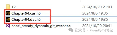
a. Open Fluent and Read CAS and DAT Files
Open Fluent and load the CAS and DAT files. The simplest 2D rectangular computational domain will suffice. Here’s an example.
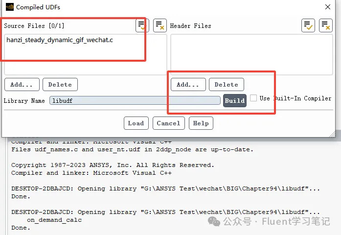
b. Compile the UDF
c. Do Not Compute the Energy Equation
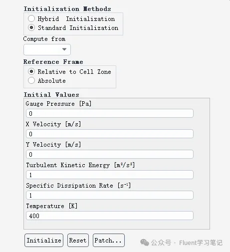
d. Standard Initialization
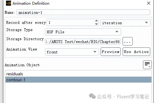
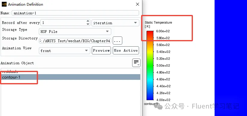
e. Generate the Temperature Cloud Plot Animation
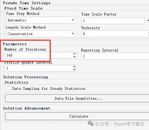
f. Change Iteration Steps to Frame Count
g. Calculation Process
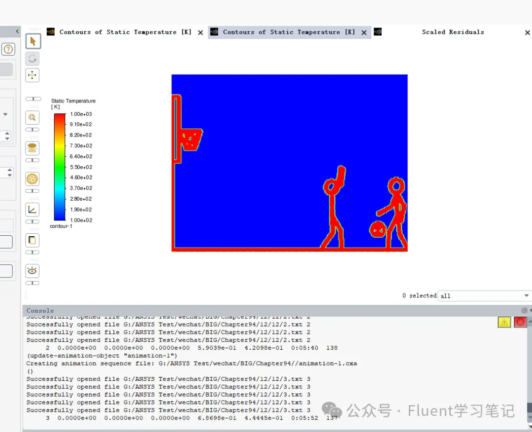
h. Generate the Final Animation
After completing the above steps, you will have the temperature animation based on the cloud plot emoji that is created by importing pixel data dynamically using UDF in Fluent.