1. Problem Description
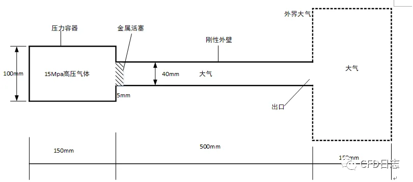
The high-pressure gas inside the pressure vessel has a pressure of 15 MPa. The gas pushes a metal piston (with a width of 5 mm) to move within a rigid pipe, from the outlet to the surrounding atmosphere.
2. Geometric Model
A two-dimensional geometric model was created using SCDM, as shown in the figure below. The geometry is simplified to a 2D symmetrical problem to reduce the computational effort.
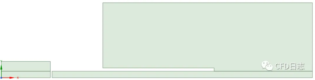
Figure: Geometric Model
Note: The computational domain is divided into several parts for ease of dynamic mesh setup.
3. Mesh Generation
The mesh was created using ANSYS Meshing, with the following steps:
- Import the geometry from SCDM into Workbench. In the main menu, select the Workbench tab, then click on WB 2020 R1 to transfer the model into Workbench, as shown below.
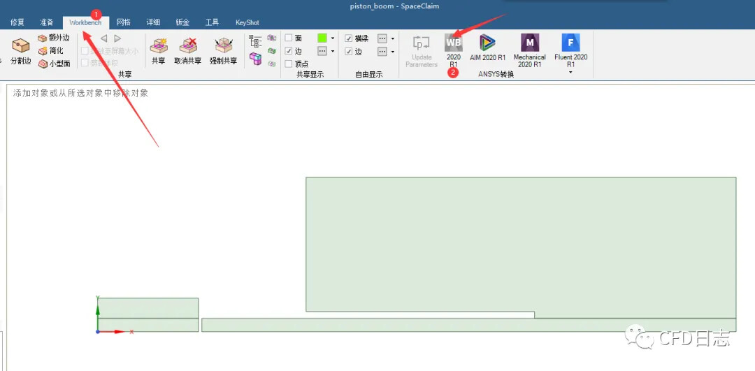
Figure: Import Geometry to Workbench
-
After starting Workbench, drag the Mesh module into the project window and activate Meshing.
-
Name the fluid domains and boundaries. The four fluid domains include:
inipressure_1,inipressure_2,piston_fluid, andfluid_out. The four solid boundaries include:piston,top,out, andout2. The three interfaces between fluid domains are:interface_piston,interface_out, andinterface_inipressure2. There is also a symmetry boundarysymm. Some of these are shown in the images below.
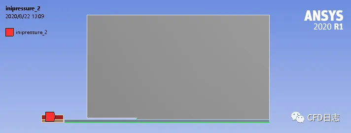
Figure: inipressure_2

Figure: inipressure_1
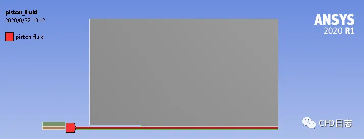
Figure: piston_fluid
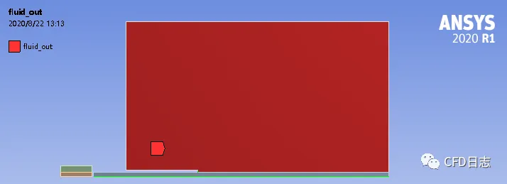
Figure: fluid_out
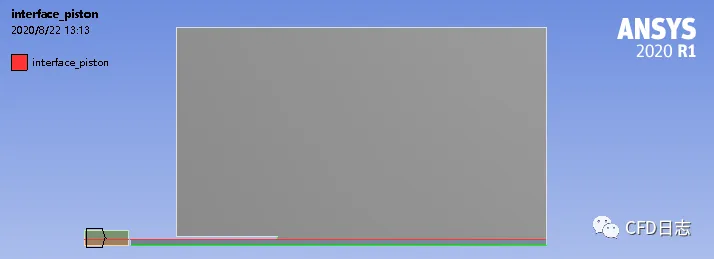
Figure: interface_piston
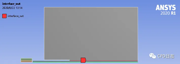
Figure: interface_out
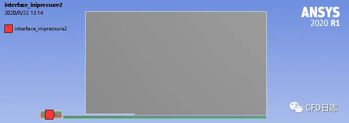
Figure: interface_inipressure2
- Mesh Generation: The mesh size in the region traversed by the piston is 2 mm, while the mesh size in other fluid regions is 4 mm. The final mesh is shown in the figure below.
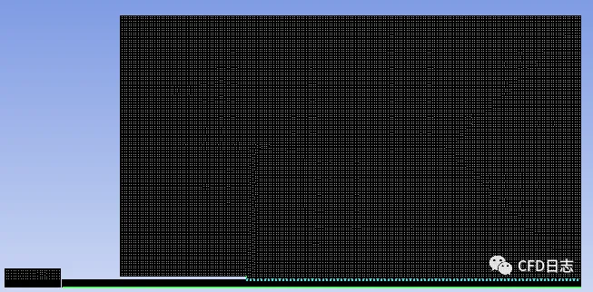
Figure: Mesh Generated
- Save the mesh in Fluent format.
4. Fluent Solution Setup
4.1 Physical Model
Enable transient solving, select the k-e turbulence model, and enable the energy equation. Since the problem involves the expansion of high-pressure gas, air is set as an ideal gas.
4.2 Boundary Conditions
The outlet boundaries out and out2 are set as pressure outlets, as shown in the figure below.
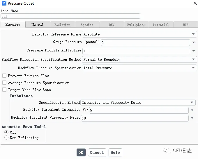
Figure: Outlet Boundary Conditions
4.3 Operating Conditions
Click on the main menu bar, select Physics → Zones → Cell Zones, and set the operating conditions in the popup window as shown below.
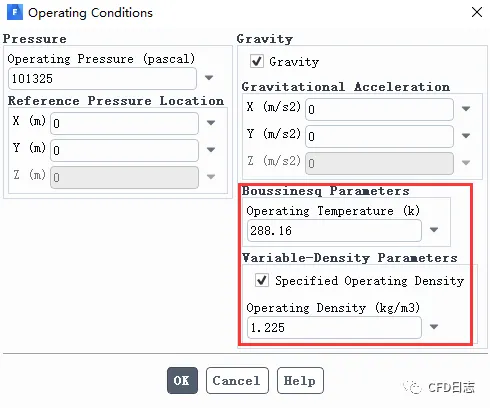
Figure: Operating Conditions Setup
4.4 Interface Settings
Manually set the interface between fluid domains as shown in the figure below.
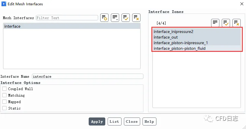
Figure: Interface Setup
4.5 Dynamic Mesh Settings
Double-click on the Dynamic Mesh in the model tree to enable Layering and Six DOF, and create the Six DOF properties as shown below.
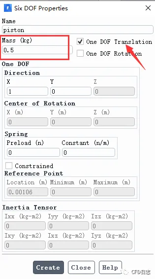
Figure: Six DOF Settings
- The dynamic mesh regions and their parameter settings are shown in the images below.
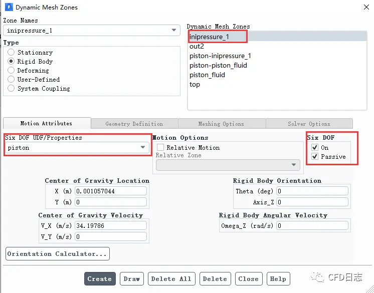
Figure: inipressure_1
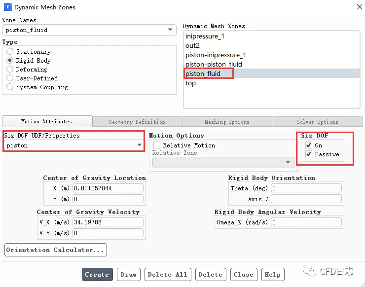
Figure: piston_fluid
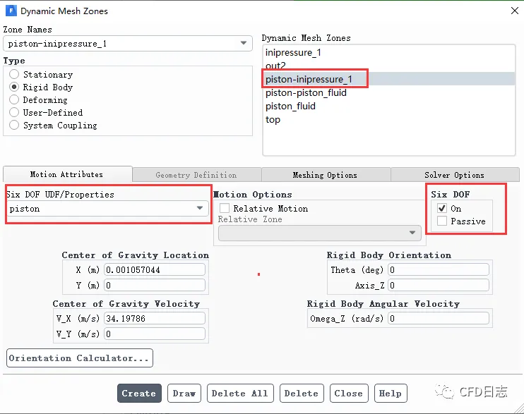
Figure: piston-inipressure_1
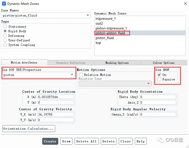
Figure: piston-piston_fluid
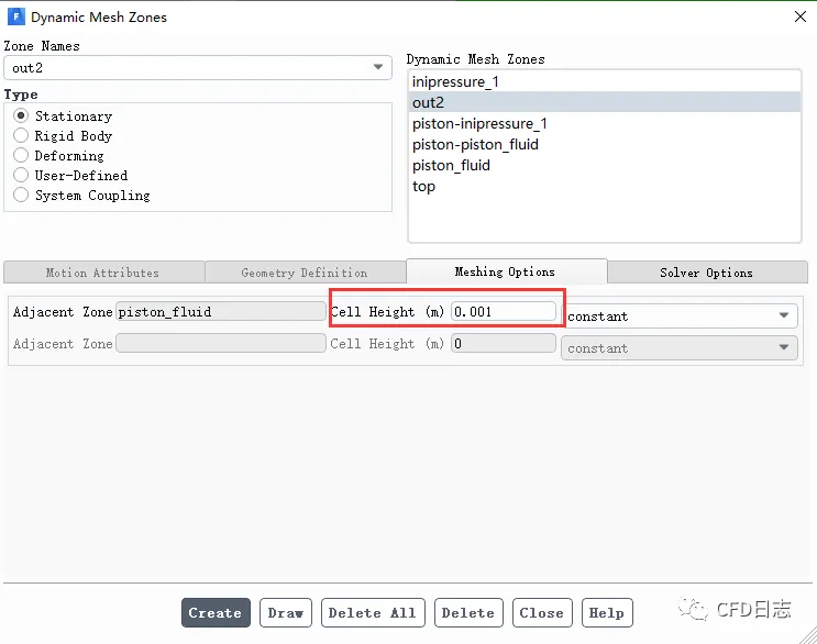
Figure: out2
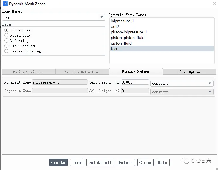
Figure: top
4.6 Initialization
Use the standard format for initialization, then set the patch as shown in the figure below.
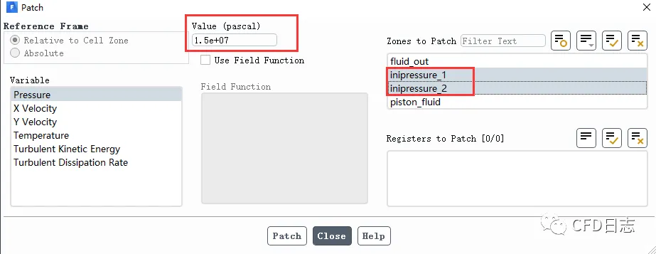
Figure: Initialization of High-Pressure Region
4.7 Calculation Settings
The calculation settings include the total number of time steps and the time step size, as shown in the figure below.
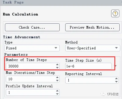
Figure: Calculation Settings
5. Result Analysis
An animation is provided, concluding the process.
Figure: Result Animation